> For the complete documentation index, see [llms.txt](https://nishanthkp.gitbook.io/tableu/llms.txt). Markdown versions of documentation pages are available by appending `.md` to page URLs; this page is available as [Markdown](https://nishanthkp.gitbook.io/tableu/chapter-3/bullet-chart-exercise-1.md).

# Bullet Chart Exercise 1

We’ll build a bullet graph using the `Chapter 3` workbook, which contains the `Hospital Visits` and `Hospital Goals` spreadsheet data sources. We’ll use these two data sources to visualize the relationship between actual and target minutes to service as you follow these steps:

1. Navigate to the **Revenue Per Department (Bullet Chart)** sheet.
2. Create a basic bar chart of the total **Revenue** per **Department**. You can accomplish this by dragging **Department** to **Rows** and **Revenue** to **Columns**.
3. Sort **Department** from highest to lowest.
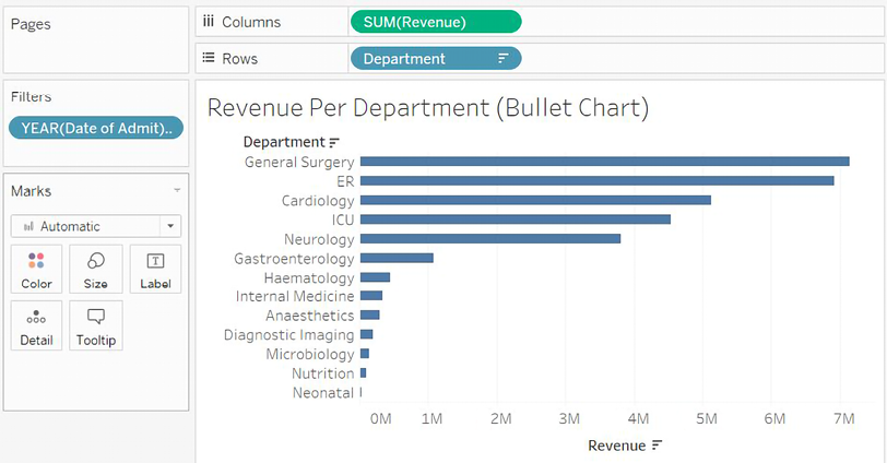
4. Filter **Date of Admit** by **Year** and keep only `2019` data. At this point, your view should look like this:

<figure><img src="https://static.packt-cdn.com/products/9781801072328/graphics/Images/B17127_03_08.png" alt=""><figcaption></figcaption></figure>

Figure 3.8: Interim steps in creating the bullet graph

1. In the **Data** pane, select the **Goal** field under the `Hospital Goals.csv` table.
2. Open **Show Me** and select the bullet graph option. At this point, Tableau will have created a bullet graph using the fields already in the view and the **Goal** field you selected in the data pane.

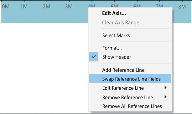
When you use **Show Me** to create a bullet chart, you may sometimes find that Tableau uses the fields in reverse order from what you intend (with the wrong measure defining the axis and bars, and the other defining the reference line). If this happens, simply right-click the axis and select **Swap Reference Line Fields**:

<figure><img src="https://static.packt-cdn.com/products/9781801072328/graphics/Images/B17127_03_09.png" alt=""><figcaption></figcaption></figure>

Figure 3.9: The Swap Reference Line Fields option

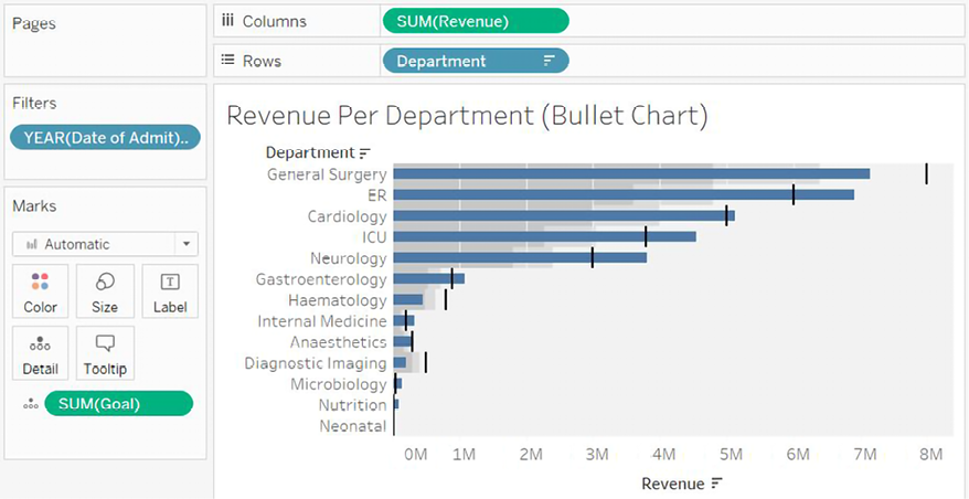
The completed bullet chart should look like the following:

<figure><img src="https://static.packt-cdn.com/products/9781801072328/graphics/Images/B17127_03_10.png" alt=""><figcaption></figcaption></figure>

Figure 3.10: The complete bullet graph

The completed bullet graph allows us to see which departments have met their goals and which are behind. Next, let’s consider how we can highlight this even more.

## **Calling out thresholds**

With bullet charts, it can be helpful to visually call out the bars that fail to meet or exceed the threshold. We’ll look at calculations in depth in the next chapter, but for now, you can complete this example with the following steps:

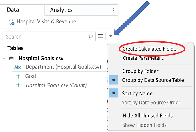
1. Use the drop-down arrow in the **Data** pane and select **Create Calculated Field…**:

<figure><img src="https://static.packt-cdn.com/products/9781801072328/graphics/Images/B17127_03_11.png" alt=""><figcaption></figcaption></figure>

Figure 3.11: Creating a calculated field

1. Name the calculated field **Goal Met?** and add the following code:

   ```markup
   SUM([Revenue]) >= SUM([Goal])
   ```
2. Click **OK** and drag the new **Goal Met?** field from the Data pane and drop it on **Color**.

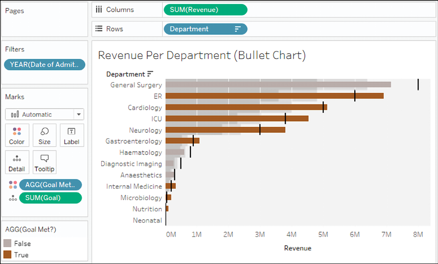
The calculation returns `true` when the `Revenue` value for a department is greater than the goal value, and `false` otherwise. With the calculated field on **Color**, it becomes very easy to see which departments have met the 2019 goals:

<figure><img src="https://static.packt-cdn.com/products/9781801072328/graphics/Images/B17127_03_12.png" alt=""><figcaption></figcaption></figure>

Figure 3.12: Departments that have met their goal are highlighted in this bullet chart

Color is one of the strongest ways to get attention with your visualizations. Use color with intent. Decide whether you want to highlight good or poor performance.